A common task when when working with data, is the recoding of values. There are many reasons you might want to do that. Maybe you want to create different groups out of one variable or just translate some responses from german to english. In this blogpost I want to demonstrate how this can be achieved in two different ways. Additionally, I will have a look at the {tidytable} package developed by Mark Fairbanks.
I feel quite at home in the tidyverse and had never really felt the necessity to deal with {datatable}. When I came across a tweet discussing {tidytable} I wanted to have a look. The reason why I don’t use {dtplyr} is that {tidytable} to my knowledge has a better support for tidy evaluation.
The {tidytable} package
To cite the first lines of the documentation page:
Why {tidytable}?
- tidyverse-like syntax built on top of the fast {data.table} package
- Compatibility with the tidy evaluation framework
- Includes functions that dtplyr is missing, including many {tidyr} functions
If you want to learn more about the package, Bruno Rodriguez has written a great blogpost introducing it. The idea is that {tidytable} functions behave more or less like classic {dplyr} or {tidyr} functions to make it as easy as possible coming from the classic tidyverse. A dot at the end of the function indicates the {tidytable} version (e.g. mutate.() and not mutate()). So let’s start and load our necessary libraries:
# Required libraries
library(tidyverse)
library(tidytable)
library(microbenchmark)

# Set custom theme for plots
plotutils::set_custom_theme(base_size = 34)
The Scenario
We’ve got several dataframes (tibble or tidytable) consisting only of one variable. For simplicity this variable is just composed of the 26 letters of the alphabet. Now I want to recode some of these letters. Like the letters, fruits are chosen here as an example completely arbitrarily. What we want to do is compare the speed of recoding some of these letters when the size of the dataframe increases. This means each dataframe has n rows and we test our different approaches with an increasing size of n. I decided to start with one thousand (1e3) rows and increase the size up to ten million (1e7) rows.
n_values <- c(1e3, 1e4, 1e5, 1e6, 1e7)
When operating on datasets with a million rows and more speed and efficient computation start to become an issue. I created the lists of dataframes by mapping over the n_values and filling the rows with letters from the alphabet.
Approach 1: left_join()
The first approach I will test is using the left_join() function from the {dplyr} package. It is basically a dictionary or look-up table to recode the values of interest. That’s why we first create the table with the information which values should be recoded to what. In this made up case an “a” and a “c” should be recoded to “apple”, the “b”, “f” and “j” to “banana” and so on. As we only want to recode some letters, we fill up the dictionary with the other distinct values in our data. Otherwise we would get an NA value for every letter that does not need to be recoded.
# Create the two dictionaries
dict_tib <- tibble(key = c("a", "b", "c", "d", "f", "j", "m", "p", "u", "y"),
               value = c("apple", "banana", "apple", "mango", "banana", "banana",
                       "mango", "papaya", "pear", "cherry")) |>
  full_join(tibble(key = letters)) |>
  mutate(value = coalesce(value, key))

dict_tidyt <- tidytable(key = c("a", "b", "c", "d", "f", "j", "m", "p", "u", "y"),
               value = c("apple", "banana", "apple", "mango", "banana", "banana",
                       "mango", "papaya", "pear", "cherry")) |>
  full_join.(tibble(key = letters)) |>
  mutate.(value = coalesce.(value, key))
Just to be consistent I use the with a dot appended {tidytable} functions. The resulting dictionary looks like this:
dict_tidyt |>
  paged_table()
Now I can define the functions to later compare in the benchmark test.
left_join_tib <- function(df) {
  df |>
    left_join(dict_tib, by = c("var" = "key"))
}

left_join_tidyt <- function(df) {
  df |>
    left_join.(dict_tidyt, by = c("var" = "key"))
}
Approach 2: case_when()
The second approach is what I’m most familiar with and my goto solution when recoding values. It uses the case_when() function inside a mutate call. Here I can easily declare what values should be recoded to.
recode_vals_tib <- function(x) {
  return(case_when(x %in% c("a", "c") ~ "apple",
                   x %in% c("b", "f", "j") ~ "banana",
                   x %in% c("d", "m") ~ "mango",
                   x == "y" ~ "cherry",
                   x == "p" ~ "papaya",
                   x == "u" ~ "pear",
                   TRUE ~ x))
}

recode_vals_tidyt <- function(x) {
  return(case_when.(x %in% c("a", "c") ~ "apple",
                    x %in% c("b", "f", "j") ~ "banana",
                    x %in% c("d", "m") ~ "mango",
                    x == "y" ~ "cherry",
                    x == "p" ~ "papaya",
                    x == "u" ~ "pear",
                    TRUE ~ x))
}
As with the second approach I create the function with a dataframe as an input to compare in the benchmark test. The small dot at the end of the functions indicates the subtle difference.
Speed comparison

Now we will use the {microbenchmark} package to compare the difference in speed when recoding values depending on the selected approach.
result <- map2_df(.x = tibble_list, .y = tidytable_list,
               .f = function(.x, .y) {
                 microbenchmark(
                   left_join_tib(.x),
                   left_join_tidyt(.y),
                   case_when_tib(.x),
                   case_when_tidyt(.y),
                   times = 50) |>
                 group_by(expr) |>
                 summarize(median_time = median(time, na.rm = TRUE))
                 })
I use the map2_df() function and give the two created lists of dataframes as an input. For each approach I test the classic tidyverse approach against the tidytable version. Afterwards I extract the median time it took. To compare the functions I plot them on a logarithmic scale on both axes.
result |>
  mutate(n_rows = rep(n_values, each = 4),
         median_time = median_time*1e-9) |>
  ggplot(aes(x = n_rows, y = median_time, colour = expr)) +
  scale_x_continuous(trans = "log10", labels = scales::label_number(big.mark = ",")) +
  scale_y_log10() +
  geom_point(size = 2) +
  geom_line(size = 1.4) +
  scale_colour_viridis_d() +
  labs(title = "Speed Comparison",
       subtitle = "X and Y Axis log transformed",
       colour = NULL,
       x = "Number of rows",
       y = "Seconds")
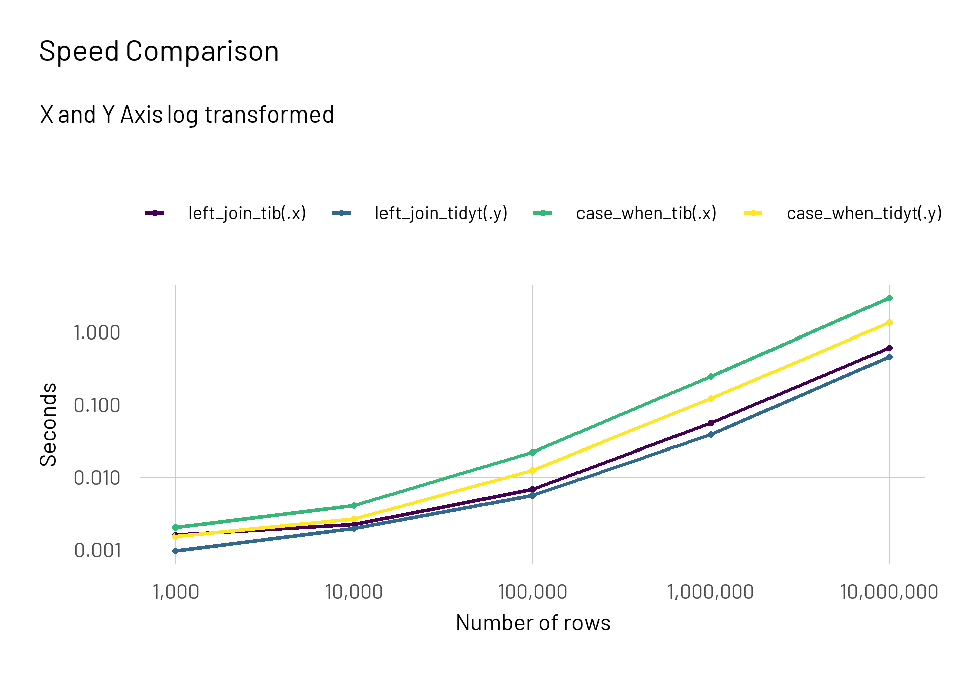
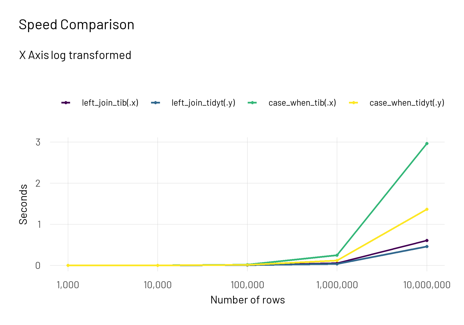
We can easily see that the {tidytable} functions outperform the classic tidyverse functions. The difference becomes more prominent when we keep the y-axis untransformed.
result |>
  mutate(n_rows = rep(n_values, each = 4),
         median_time = median_time*1e-9) |>
  ggplot(aes(x = n_rows, y = median_time, colour = expr)) +
  scale_x_continuous(trans = "log10", labels = scales::label_number(big.mark = ",")) +
  geom_point(size = 2) +
  geom_line(size = 1.4) +
  scale_colour_viridis_d() +
  labs(title = "Speed Comparison",
       subtitle = "X Axis log transformed",
       colour = NULL,
       x = "Number of rows",
       y = "Seconds")
Conclusion
For the case of 10 million rows the dplyr::case_when() approach took around 3 seconds whereas the fastest approach was the tidytable::left_join() approach with \(0.46\) seconds (more than 6 times the difference). When compared directly the dplyr::left_join() took at 1 million rows \(45.5\%\) and at 10 million rows \(31.5\%\) longer than the {tidytable} alternative.
In general the results show that when operating with dataframes of around 10 thousand rows the differences are negligible. Only when the data you are dealing with becomes significantly larger (more than 1 million rows) it is more reasonable to use the {tidytable} alternative. Furthermore, the left_join() variant is probably a bit cleaner or better to manage as you store the dictionary in a separate table. The great thing about {tidytable} is that the switch is so easy.