A few weeks ago I did an introductory R workshop where one of the students asked about loops and the difference of for vs while loops. This blogpost is about illustrating these two types of loops using a simulation example.
Let the Game begin
I think the majority knows the Netflix show “Squid Game”. In this series the contestants have to survive several deadly games. Here I want to focus on the 5. game of the show. There are 16 players who have to pass a bridge of 18 * 2 glass plates. At each step they have to decide on which plate they step. With a 50% chance they jump on the harder glass which is able to hold their body, the other 50% will mean their death. As I was watching the show I thought that this would be a perfect example to answer a statistical question by using loops and simulation.
The question I wanted to answer was:
How many players do we expect to survive the game?

Figure 1: Source: https://www.distractify.com/p/games-played-in-squid-game
Remark:
After opening twitter, I came across a tweet discussing John Helveston’s blogpost where he basically explained exactly what I wanted to do. I highly recommend his blog. I adapted his run_game function and where he used data.table I went with the tidy alternative.
Monte Carlo Solution
We can solve the question about the number of survivors to expect by simulating the game. When using random simulation to answer statistical problems, this is called Monte Carlo Simulation.
First we load the necessary library and set a custom theme for our plots.
library(tidyverse)
library(microbenchmark)

plotutils::set_custom_theme(base_size = 32)
Then we create a dataframe as an input for the game. In this dataframe the alive column is set to 1 as in the beginning obviously every player is alive.
# Define number of players
num_players <- 16
players <- tibble(player = seq(num_players),
                  alive = 1)

# Let's have a look at the dataframe
players
# A tibble: 16 x 2
   player alive
    <int> <dbl>
 1      1     1
 2      2     1
 3      3     1
 4      4     1
 5      5     1
 6      6     1
 7      7     1
 8      8     1
 9      9     1
10     10     1
11     11     1
12     12     1
13     13     1
14     14     1
15     15     1
16     16     1
Now we are going to create the function for our game. This is a great example to look at the differences between for and while loops.
We start by creating a function using a for loop:
# Define a function for simulating one game using a for loop
run_game_for <- function(players, num_steps) {
  lead_player <- 1
  for (step in seq(num_steps)) {
    # 50% chance that the glass is safe
    if (sample(c(TRUE, FALSE), 1)) {
      # It is safe, now the player can try the next one!
      next
    } else {
      # The glass broke...
      # Before continuing, check if any players are still alive
      if (sum(players$alive) == 0) { return(0) }
      # The lead player died
      players$alive[lead_player] <- 0
      lead_player <- lead_player + 1
    }
  }
  return(sum(players$alive))
}
Then we create a function using a while loop. The setup is quite similar to the previously used run_game_for function.
# Define a function for simulating one game using a while loop
run_game_while <- function(players, num_steps) {
  # Initialize starting values
  lead_player <- 1
  current_step <- 0
  game_running <- TRUE

  while (game_running) {
    # Let's see if the glass holds...
    if (sample(c(TRUE, FALSE), 1)) {
      # The glass holds and the player can go one step further
      current_step <- current_step + 1
    } else {
      # Check if there are still players alive, if not end the game
      if (sum(players$alive) == 0) { return(0)}
      # Apparently the glass didnt hold and the current lead player dies
      players$alive[lead_player] <- 0
      lead_player <- lead_player + 1
      # Anyway the player can go one step further
      current_step <- current_step + 1
    }
    if (current_step == num_steps) {
      # If they got to the last step, they did it and the game stops
      game_running <- FALSE
    }
  }
  # Return the number of remaining players
  return(sum(players$alive))
}
Let’s give it a try and see how many survive in our game.
set.seed(001)

# Run one iteration of the game
single_game <- run_game_while(players, num_steps = 18)
single_game
[1] 9We were interested in the expected value of the outcome. One iteration is not enough, but this is no problem at all. We can simply simulate our game multiple times.
# Set seed value to keep reproducibility and to give a hint who wins the game
set.seed(456)

# Define number of runs or games we want to play
n_runs <- 10000

# Create dataframe with outcome of each game
sims <- tibble(trial = seq(n_runs)) |>
  rowwise() |>
  mutate(while_loop = run_game_while(players, num_steps = 18),
         for_loop = run_game_for(players, num_steps = 18)) |>
  pivot_longer(-trial, names_to = "loop")
Have a look at the descriptive statistics:
summary(sims$value)
   Min. 1st Qu.  Median    Mean 3rd Qu.    Max.
  0.000   6.000   7.000   6.976   8.000  15.000
There were games where zero players survived the game and there were games where almost all players managed to survive.
Of course we can also visualize our distribution:
# Visualizing the resulting distribution
sims |>
  ggplot(aes(x = value, fill = loop)) +
  geom_bar(position = position_dodge()) +
  scale_x_continuous(breaks = seq(0, num_players)) +
  labs(title = "Distribution of numbers of surviving players",
       x = "N surviving players",
       fill = NULL)
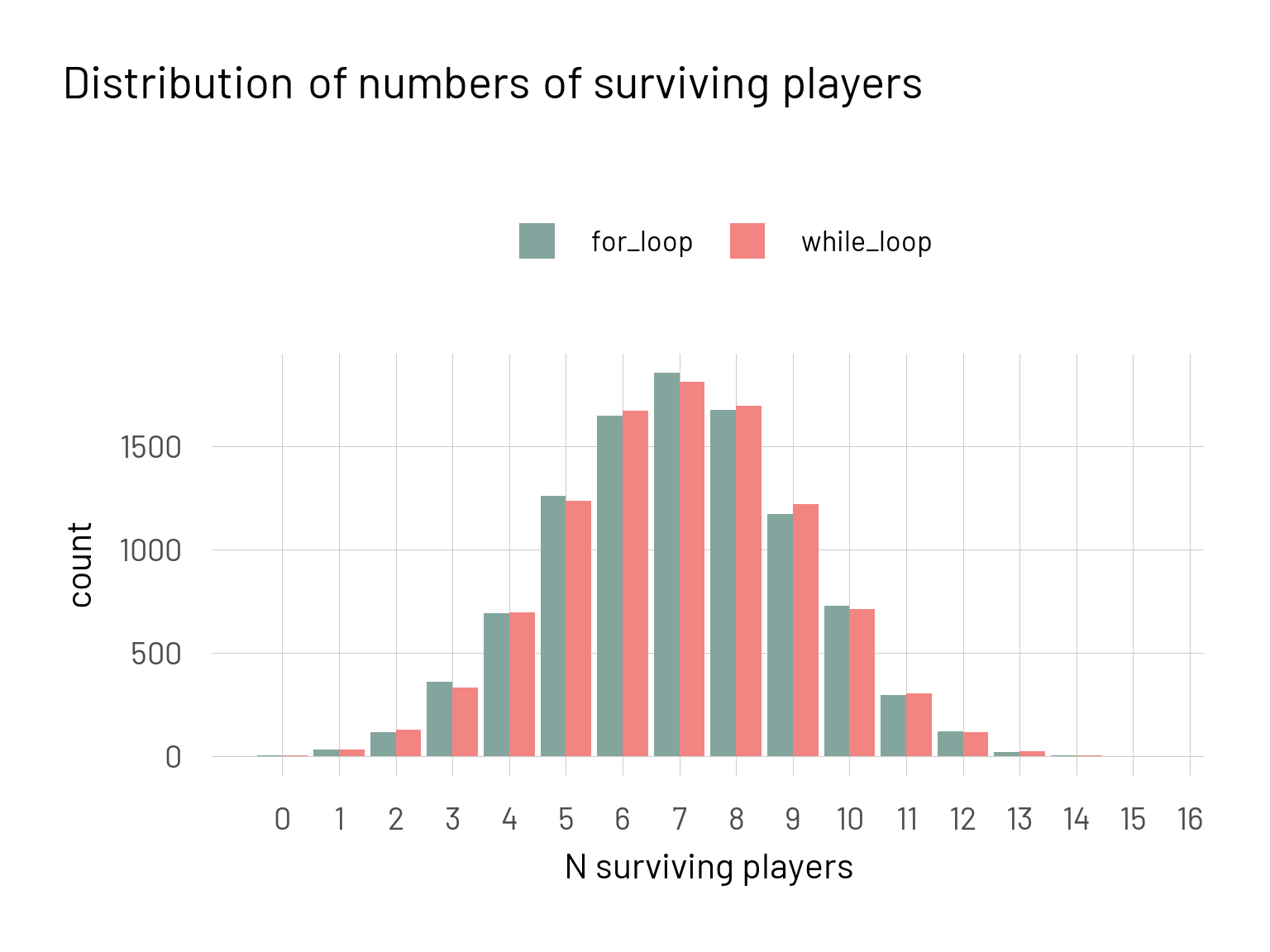
The two different colours indicate which function was used to calculate the result. From this graph we directly see almost the exact same result from the two functions.
To answer our previously posed question: We would expect 7 players to survive the game.
Benchmarking for vs while loop
Now we can also test the performance of the different functions against each other.
set.seed(001)

test <- microbenchmark(
  run_game_for(players, num_steps = 18),
  run_game_while(players, num_steps = 18)
)

autoplot(test)
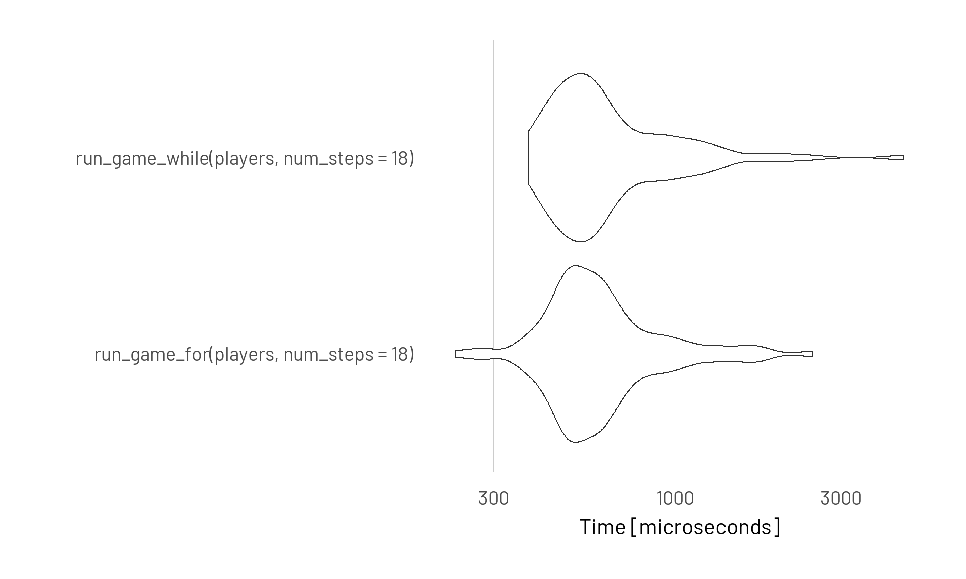
Again there is not really a difference…
Mathematical Solution
Of course we can not only simulate the game to get to our solution.
Here is the mathematical formula for n players:
\[ \sum_{i = 0}^{n-1} \binom{18}{i} * 0.5^i * 0.5^{18-i} * (n-i) \]
We can convert it to R Code and calculate the result.
n <- 16

expected_fun <- function(i) choose(18, i) * 0.5^i * 0.5^(18-i) * (n - i)

map_dbl(0:(n-1), expected_fun) |> sum()
[1] 7.000076Et voilà! The result from the Monte Carlo simulation was confirmed.